Utilities are usually among the top three operating expenses at a multifamily community, but they are also among the most complex to forecast.
For budgeting exercises of any kind, it often makes sense to first identify what you will use as your baseline, and then identify which adjustment factors will be applied. But budgeting for utilities can involve more work than budgeting for other transaction types because the potential adjustment factors involve several moving parts. They include vendor rate changes, usage changes due to operating and asset conditions, and usage changes due to weather.
Baseline Dollars
Many companies start with a simple baseline of prior year actuals. One challenge to this is that normally when budget season is upon us, Q4 actuals aren’t available for the current year —because Q4 hasn’t happened yet! Sometimes this causes a default back to the “prior prior” year actuals, but logically this implies a two-year gap between the baseline and next year’s Q4 budget. Some companies use a recent Q4 forecast, while others stick with the two-year gap and the prior year actuals. Whatever you choose, best practices include being consistent and providing clear documentation/ disclosure to all stakeholders.
Adjusting for Vendor Rate Changes
After identifying your baseline, you have several options when deciding which adjustment factors to apply. Rate changes can be treated as a simple high-level overview by using a flat-rate national average, which will be discussed further below. A more granular approach, if you have already collected rate notices throughout the year or can set aside time to research by calling vendors and searching vendor websites, is to apply a different rate for each of your vendors based on published vendor rate changes. Some utility management companies also offer this rate research service for a fee. The output of these services range from a simple PDF booklet organized by vendor to a detailed Excel file with rates conveniently linked to each of your properties. Lastly, if you participate in energy procurement contracts in deregulated markets, ask your broker or supplier for property-specific price change guidance that is customized with the actual pricing you have locked in.
Flat-Rate National Averages
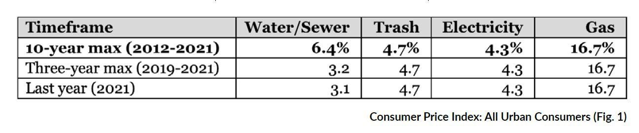
Average U.S. price increases for different types of utilities are shown in Fig. 1. Some like to use the first row because it is a likely worst-case scenario, showing the highest annual increase in the last 10 years (2012- 2021). In the case of water and sewer for example, while the average annual increase over last year was 3.1%, the highest increase over the same period was 6.4%. In addition to the more conservative worst-case approach, there are three-year max and last year increases shown, which could be used instead. In the case of trash, electricity, and gas, last year was the highest increase during the last 10 years thereby resulting in the unusual situation of all three rows having the same value for these columns!
Note that Fig. 1 shows historical performance. As they say on Wall Street, past performance is not necessarily indicative of future results. That said, in the case of water/sewer and trash, this is probably a good gauge for setting future expectations.
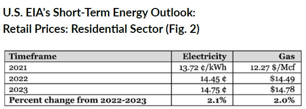
Since energy (electricity and natural gas) tend to be more volatile, many property and asset managers ignore historical averages and instead use the U.S. Energy Information Administration (EIA’s) forecasts for residential retail price increases for the coming year. Their latest numbers are shown below (Fig. 2), and in this case are surprisingly less conservative than the historical numbers above.
Note that EIA releases an updated outlook around the same time each month. This article is based on the June 7, 2022, release. If you can wait to finalize your budget until a later update, it might make sense to use their current numbers as a placeholder and refresh your budget when the new numbers are published. You can always find EIA’s latest outlook at: eia.gov/steo.
Rate Adjustments Wrap-Up
You may have heard the saying, “it’s a budget, not a Bible.” If you subscribe to this philosophy and prefer to keep your adjustment factors simple, then you might want to pick one of the flat-rate national average methods mentioned above, multiply it against your baselines and stop right there. There is certainly value to that approach, not the least of which is producing numbers that are easy to understand and explain/defend during your internal budget review meetings. But for those of you who are on a quest for the holy grail of trying to produce a budget that most accurately tracks with next year’s actual expenses, you may decide to apply more vendor-specific adjustments, as well as reading on to include additional types of usage adjustments.
Adjusting Usage for Operational Changes
In order to determine the impact of operating and asset changes, you’ll need to research that on a property-by-property basis. At this stage, you are looking to catalog the impact of issues that could impact your utility expenses or revenues, such as capital improvement projects, resident billing or other policy changes, and occupancy rates. You should note any anomalies that may have occurred in the prior year.
Adjusting Usage for Weather
When considering usage assumptions based on weather, many use it as a sanity check rather than a detailed adjustment factor. In order to evaluate the impact of weather on utility usage, it is worth considering the temperatures during both the baseline period and the forecast period. Did the baseline period experience near normal temperatures, and is the forecast period expected to be near normal? In many parts of the United States, extreme weather seems most frequent during summer (June, July and August) and winter (December, January and February). The National Weather Service publishes average temperature information that can be used as a reference when reviewing weather conditions. They define “normal” using 30-year averages. You can get a ballpark sense of prior and forecast temperatures by comparing Fig. 3 with Fig. 4 for summer and comparing Fig. 5 with Fig. 6 for winter. Note that these maps do not show percentage variance but rather show degrees Fahrenheit anomaly for prior period, and simply show whether an area is likely to have above, below or normal temperatures for the future period.
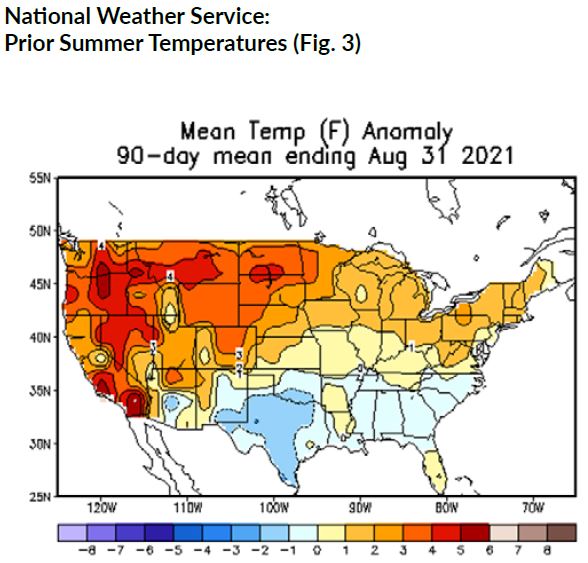
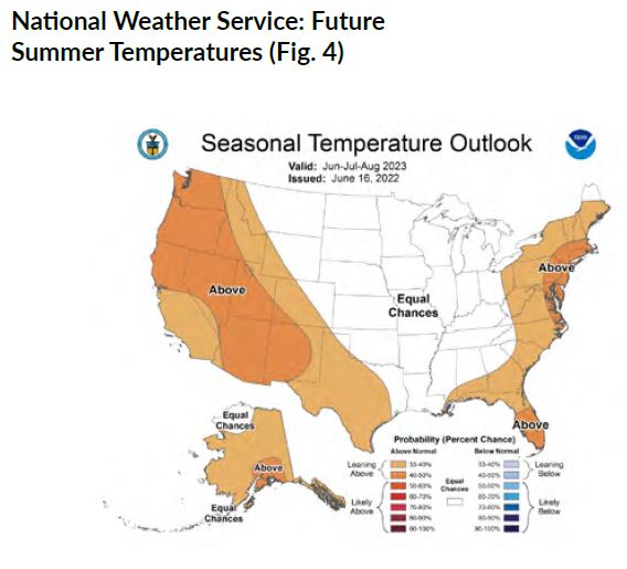
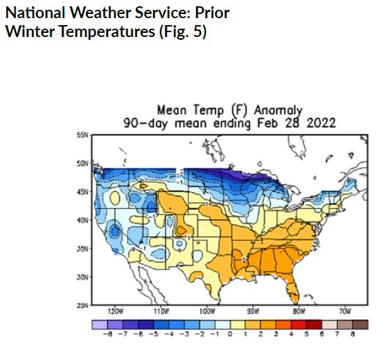
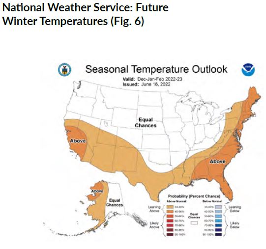
For example, according to Fig. 5 the prior winter in Georgia was above normal (unusually warm). Taken by itself, one might want to budget an extra increase in heating costs for the coming winter. However, according to Fig. 6 the future winter is also leaning toward having above normal temperatures, which may make a special weather adjustment unnecessary for any properties in Georgia. On the other hand, Fig. 3 shows the prior summer in Texas was below normal (unusually cool) and Fig. 4 shows the future summer could bring above normal (unusually hot) temperatures to most of the state. Budgeting an extra increase for properties in this location (in addition to any rate or other adjustments) could be helpful.
Calculating a specific percentage for weather adjustment can be difficult. This aspect is more of an art than a science as illustrated by the examples above. While it is possible to obtain data on prior weather versus normal weather for each of your locations, trying to quantify future weather is generally elusive.
As we have seen, budgeting for utilities involves many considerations, but there are methods, resources, and data available to make the process more bearable. Identify baselines and then adjust for significant changes in vendor rates, operations, assets and weather.